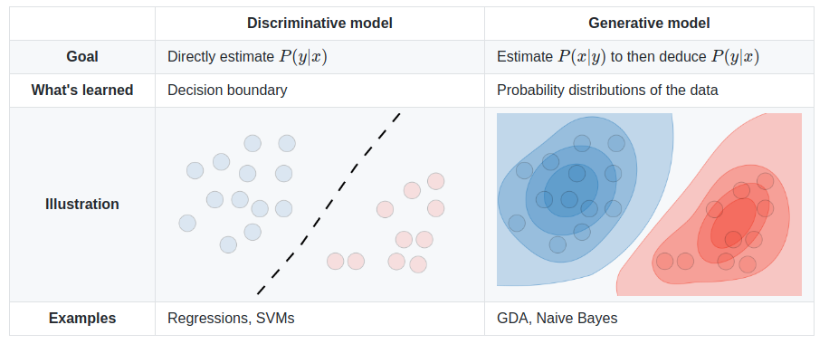
A type of regression model (like Linear Regression) but where the dependent variable (the thing being predicted) is categorical, rather than continuously varying over a range. For example, Logistic Regression might be used to predict if a house split level or ranch based on the number of rooms, where linear regression would be used to predict something like the value or selling price. It discriminates between groups of data, but does not generalize either the best seperation between the groups, nor does it find the probable center or distribution of the groups. It works well and inexpensively when the data is spread out but has a clear and linear boundry. When the boundry is non-linear, or some (training) data may be spread away from the actual boundry, an SVM may work better. When the data is clustered or grouped, a Bayesian Classifier may work better.
Although the prediction is binary, the model uses a Percentage Chance
Prediction for each possible outcome. E.g. what is the percentage chance
that a house is split level given that it has 5 rooms? So 0 <
ho(x) <= 1. The probability that y=1, given
x parameterized by o, can be written
as: ho(x) = P(y=1:x;o)
Assuming that y can only be 0 or 1, if P(y=1:x;o) =
0.7, then we know there is a 70% chance that y is 1. There is then, obviously,
a 30% chance that y is zero, or P(y=0:x;o) = 0.3.
I.e. the total probabilities must add to 1.
As expected, our job is to find o such that x is transformed
into a valid prediction of the probability that y is 1. We can then apply
a Decision Boundary which divides the probability into a 1 or 0. For
example, we might say that y is 1 when the probability of y being 1 is higher
than 50%. So our hypothesis function needs to translate values of
OTx such that
g(OTx) will be >= 0.5 when
OTx >= 0 (positive) and less than 0.5 when
OTx < 0 (i.e. negative) but the result will
never be more than 1 or less than -1.
 Rather
than use a hypothesis funciton of
Rather
than use a hypothesis funciton of OTx as
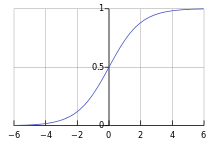
in Linear Regression, we need to use the Logistic Function
^
g(OTx) where g(z) is:
1 |
|
|
| 1+e-z |
which is also called the Sigmoid Function^. In Octave:
function g = sigmoid(z)
%SIGMOID Compute sigmoid functoon
%   J = SIGMOID(z) computes the sigmoid of z.
% (z can be a matrix, vector, or scalar).
  g = 1 ./ ( 1 .+ exp(-z) ) ;
  end
This sigmoid function simply limits our result into the maximum range we
desire, with a rapid transition at OTx = 0.
Note: The decision boundary may not be a straight line if the hypotheses includes terms which define other terms. E.g. x2
Cost Function: The standard Mean Squared Error
(MSE)^ function
doesn't work well as a cost function for sigmoid because it results
in graph that is not convex, but instead is "pitted" with many local minima.
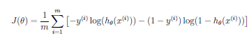
Instead we use:
-log(ho(x)) if y = 1
-log(ho(x)) if y = 0
This produces a nice curve that, when y = 1, slowly approaches 0 as
ho(x) approaches 1 yet quickly becomes infinite
near zero 0 and does exactly the opposite when y = 1, i.e. it slowly approaches
0 as ho(x) approaches 0, but quickly become infinite
as it approaches 1. This gives us near infinate cost as our error is large,
and very little change in cost as our error decreases toward zero, helping
us to not overshoot our goal. Also, the relationship between the loss function
and the parameters w still gives us a concave error function. Thus, we can
rest assured that there is only a unique minimum on the error surface.
We can combine the two cases (y=0 or y=1) into one equation by multiplying one side by y and the other side by 1-y; which ever term is unwanted, will be multiplied by zero and drop out.
hO(x(i)) =
g(OTx(i))
Hypothesis Function: If we transpose each x(i) and build
a matrix X =
[(x(1))T;(x(2))T;...(x(m))T]
given O =
[O0;O1;...On]
then the matrix product XO is
[OTx(1);OTx(2);...OTx(m)].
In other words, if we build a matrix X (note the capital X vs x) where each
row is a set of input values (x(i))T), then
OTx(i) becomes XO
which is a vector with each element being the sum of the values of
O times each input. We can then take the sigmoid function
of each row to form our vector of hypothesis values. In
Octave:
hyp = sigmoid(X*theta);
Calculating our cost then becomes simple matrix math by taking the transpose of the y values or the (1-y) values times the hypothesis or 1 - hypothesis vector. In Octave:
errs = -y' * log(hyp) - (1-y)' * log(1-hyp);
The cost for a given set of parameters over the training set is then simply the sum of the costs divided by the number of errors. In Octave:
J = sum(errs)/m;
Slope Function: As with the MSE in Linear Regression, the Sigmoid
function has a very simple derivative
ho(x(i) - y(i)) *
xj(i) (it's quite difficult to take the derivative
of it, but once you do, the result is this very simple equation) which makes
it easy to calculate the slope of the error. This makes the gradient descent
quick, which is why we picked it in the first place. Just like in Linear
Regression we do:
Oj := Oj - a * sum
i=1 to m (
(ho(x(i)) - y(i)) *
xj(i) ) / m
We have already calculated our
ho(x(i)) for all i as
XO which is a vector. The error is then that value less
our known values of y. ßi =
ho(x(i)) - y(i) or in Matrix
form ß = XO - y which is still just a vector. In
Octave:
err = (hyp .- y)
To multiply by xj(i) and sum, understand that we are calculating sum(ßi x(i)) where x(i) is a vector (one set of inputs) and ßi is a scaler (one hypothesis less the actual y value for that input). Multiplying each x(i) vector times each ßi and summing the output, is the same as Matrix multiplying the transpose of X by the vector of scalers ß.
sum(ßi x(i)) = [x(1) x(2) ... x(m) ] * [ß1 ; ß2 ; ... ßm ] = XTß
Gradient Decent: Keeping in mind that we must simultaneously update
all O and that hO is now a totally
different equation based on the sigmoid function.
% Basic Logistic Regression via gradient decent with multiple parameters in Octave
alpha = 0.01; % try larger values 0.01, 0.03, 0.1, 0.3, etc...
m = length(y); % number of training examples
p = size(X,2); % number of parameters (second diminsion of X)

for iter = 1:num_iters %for some number of iterations
  hyp = sigmoid(X*theta); %calculate our hypothesis using current parameters
  err = (hyp .- y); %find the error between that and the real data
  s = sum( err .* X )./m; %find the slope of the error.
  %Note: This is the derivative of our cost function
  theta = theta - alpha .* s;
  %adjust our parameters by a small distance along that slope.
  end
Not all data fits well to a straight line. This is called "underfitting"
or we may say that the algorithm as a "high bias". We can try fitting a quadratic
or even higher order equation. E.g. instead of
O0 + O1x, we might
use O0 + O1x +
O2x2. But, if we choose an equation
of too high an order, then we might "overfit" or have an algorithm with "high
variance", which would fit any function and isn't representing the function
behind this data. Overfitting can therefore result in predictions for new
examples which are not accurate even though it exactly predicts the data
in the trianing set. The training data may well have some noise, or outliers,
which are not actually representative of the true function.
If the data is in 2 or 3 features, it can be plotted and a human can decide if it is being over or under fit. But when there are many parameters, it can be impossible to plot. And using a human is sort of against the purpose of Machine Learning. It may help to reduce the number of features if we can find features that don't really apply. Another means of reducing overfitting is regularization.
To keep the system from over fitting, and instead provide a more generalized fit, we can add the sum values of the theta parameters to the cost and slope of the error. Here is that new term added to the right of our cost function:

Question: Shouldn't we use lower weight parameters (more regularization) for higher order terms?
Don't regularize O0.
Lambda is used as a parameter for the amount of regularization. e.g. the amount that the parameter values are multiplied by before adding them to the cost function. To large a lambda can result in underfitting.
reg = lambda * sum(theta2.^2) / (2*m);
J = J + reg;
...
reg = lambda .* theta2 ./ m ;
S = S + reg;
Where theta2 is either:
theta2 = theta;
theta2(1) = 0;
Or
theta2 = [0; theta(2:end)]
(the [0; and ] aren't needed for the cost calculation, only for the gradient / slope.
Find Minimum Function: fminunc( @[cost, slope] = cost(theta, X, y), theta, options )
But there are better (and more complex) means of adjusting the theta (parameter) values to minumize cost. fminuc is a common and powerful method. The fminunc function expects a reference to a function which will return cost and (optionally) slope / gradient values for a given set of parameters, training data, and training answers. It starts from an initial set of parameters and there are some options which can be set, such as the maximum number of iterations.
Here is a complete learning function in Octave using fminunc:
function [J, S] = costSlope(theta, X, y, lambda)
%return cost (J) and slope (S) given training data (X, y), current theta, and lambda
  m = length(y);
  hyp = sigmoid(X*theta);
  %make a guess based on the sigmoid of our training data times our current paramaters.
  costs = -y' * log(hyp) - (1-y)' * log(1-hyp); %costs with sigmoid function
  %costs = -y .* log(hyp) - (1-y) .* log(1-hyp); %more general version?
  J = sum(costs(:))/m; %mean cost. (:) required for higher dimensions
  reg = (lambda * sum(theta(2:end).^2) / (2*m)); %mean cost + regularization
  J = J + reg; %add in the regularization
  err = (hyp .- y); %actual error.
  %Note this happens to be the derivative of our cost function.
  S = (X' * err)./m; %slope of the error
  reg = lambda .* [0;theta(2:end)] ./ m; %Also regularize the slope
  S = S + reg; %add in the regularization
  end

options = optimset('GradObj', 'on', 'MaxIter', 400);
[theta, cost] = fminunc(@(t)(costSlope(t, X, y)), initial_theta, options);
For more about the @(t) () syntax see Octave: Anonymous Functions
Also: fmincg. This works similarly to fminunc, but is more efficient when we are dealing with large number of parameters.
It's very easy to turn this into a "one hot" logistic classifier
Also:
See also:
| file: /Techref/method/ai/logisticregresions.htm, 15KB, , updated: 2019/3/6 12:12, local time: 2025/6/1 09:37,
216.73.216.214,10-3-106-20:LOG IN
|
| ©2025 These pages are served without commercial sponsorship. (No popup ads, etc...).Bandwidth abuse increases hosting cost forcing sponsorship or shutdown. This server aggressively defends against automated copying for any reason including offline viewing, duplication, etc... Please respect this requirement and DO NOT RIP THIS SITE. Questions? <A HREF="http://www.sxlist.com/techref/method/ai/logisticregresions.htm"> Machine Learning, Artificial Intelligence Method, Logistic Regression</A> |
| Did you find what you needed? |
Welcome to sxlist.com!sales, advertizing, & kind contributors just like you! Please don't rip/copy (here's why Copies of the site on CD are available at minimal cost. |
Welcome to www.sxlist.com! |
.