The percentage that are miss-classified is called the "0/1 misclassification error" metric. Diagnostics can take time, but give a clear direction to proceed. In fact, instead of trying to intuit the best system, it is often best to start with a very basic, very quick system that doesn't work well, but will provide a starting point for diagnostics to lead you to a better system. Use your intuition to find better features, interactions, or to try to see the pattern in mistakes. Test each model change against the validation data to find out which is better.
Training, Validation, and Test Data: Always use part, randomly selected, of your training example set as a test set. Train on part and test against the rest. By definition, the training error is only valid for the training data. If the fit is valid, you will find it works well for the test data as well. Without the separate test data, you may think you are getting a good fit when you are not.
When trying multiple models, with different number of features, or polynomials, or Lambda, or whatever, split the data into 3 parts:
Train all test models on the training set. Test each model against the validation set. Select the best model and test against the final test set.
 Bias vs Variance:
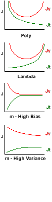
As we increase the number of polynomials, our training
error Jt decreases, and our validation
Jv (and test) errors will initially also decrease, then
increase again as we begin to over fit. While both are decreasing, we are
under fitting. This is "Bias". (left side of top graph). When training error
is decreasing, but test error is increasing, we are over fitting. This is
"Variance". (right side of top graph)
As we increase the Lambda regularization, our training error Jt increases, and our validation Jv (and test) errors will initially decrease, then increase again as we begin to under fit. While both are increasing, we are under fitting. This is "Bias". (right side of bottom graph). When training error is increasing, but test error is decreasing, we are over fitting. This is "Variance". (left side of bottom graph)
High Bias: (e.g. too few polynomials, too little regularization) If you start with very few training examples (m), and increase your dataset, the training error will start low (it's easy to fit a few points with any model) then quickly increase and level off as the fit can't match the new data. At the same time, the validation / test error will start very high and then decrease but never pass below the training error. Starting with a small subset of the training data, and then increasing that set while tracking training and validation errors, can diagnose the High Bias case.
High Variance: (e.g. too many polynomials, too much regularization) As the training set size increases, the training error will start and remain low (perhaps increasing a little). But the validation error will start high, stay high, and never come down to the training set error. When we track the errors as the size of the training set increases, and we see this curve, we know we are in the High Variance case. However: If the validation error is continuing to decrease, it may be that we simply need more training data, and that the data we have is "noisy" or that the function is very difficult to fit.
%in Octave
lambda_vec = [0 0.001 0.003 0.01 0.03 0.1 0.3 1 3 10]; %known good values
error_train = zeros(length(lambda_vec), 1);
error_val = zeros(length(lambda_vec), 1);
X = [ones(size(y), 1) X]; %no need to do this each time
Xval = [ones(size(yval), 1) Xval]; %no need to do this each time
for i = 1:length(lambda_vec)
    lambda = lambda_vec(i);
    theta = train(X, y, lambda);
    error_train(i) = cost([ones(size(y), 1) X], y, theta, 0);
    %note lambda is passed as 0 here to give the true cost.
    error_val(i) = cost(Xval, yval, theta, 0);
    %note we check against ALL the validation data.
    end
%in Octave
m = size(y);
error_train = zeros(m, 1);
error_val   = zeros(m, 1);
Xval = [ones(size(yval), 1) Xval]; %no need to do this each time
for i = 1:m
    Xsub = X(1:i,:); %cut out the first ith examples
    ysub = y(1:i);
    theta = train([ones(i, 1) Xsub], ysub, lambda);
    error_train(i) = cost([ones(i, 1) Xsub], ysub, theta, 0);
    %note lambda is passed as 0 here to give the true cost.
    error_val(i) = cost(Xval, yval, theta, 0);
    %note we check against ALL the validation data.
    end
Note: In the above code samples train(X, y, lambda) is a function which must be provided to train the system using those parameters. Similarly, cost(X, y, theta, lambda) should return the cost (and probably the slope for use in training) for the current theta and other parameters.
function [F] = polyFeatures(X, p)
for i = 1:p; %for each new order of poly
  F(:,i) = X .^ i; %add a new column of Xp
  end %note .^ not ^
Making these changes gives you new models. Finding the best model is called Model Selection.
Smaller Neural Networks are easier to compute and much easier to train. NN with a large number of nodes, while expensive, generally work better; they can over fit, but that can be addressed by higher Lambda.
One cheap way of combining different words (e.g. "fishing", "fished", and "fisher" are all about "fish") is using only the first few letters of each word and is called "stemming". Search for "Porter stemmer" for more.
Prevalence: The actual likelihood of some fact being true in the population. E.g. "1 in 12 dogs have fleas" or "the rate of sexual abuse of girls is 20%". It is very important to note that prevalence can be very difficult to know with certainty in the real world. We usually estimate prevalence by sampling a statistically significant subset, which gives us an answer very likely to be correct. In machine learning, we rely on accurately labeled training data, and that may not be infallible, unless we have generated the training data ourselves. Using auto-generated data vs collected data is a good troubleshooting technique to detect poorly labeled data.
Skewed classes: When you have a low prevalence, far more examples of one output vs another. E.g. when only 0.5% of your examples is in a given class when y=1 vs 0. It can be very difficult to know if your error calculation is actually working. Just predicting that the output isn't in that class, always predicting y as 0, can be more accurate than a real test! Instead of accuracy, use Precision/Recall. Use Bayes Rule to check that your predictions are significant in a skewed population.
| Actual Class y= |
|||
| 1 | 0 | ||
| Predicted Class |
1 | True Positive |
False Positive I |
| 0 | False Negative II |
True Negative |
|
I False Positive is a "Type I error" aka "error of the first kind",
"alpha error". It is hypochondria, excessive credulity, hallucination, false
alarm, or "crying wolf"
II False Negative is a "Type II error" aka "error of the second
kind", "beta error". It is denial, avoidence, excessive skepticism, myopia,
or "ignoring the gorilla in the room"
In Octave:
true_positives = sum((predictions == 1) & (y == 1)); %we predicted true, and it was
true_negatives = sum((predictions == 0) & (y == 0)); %we predicted false, and it was
false_positives = sum((predictions == 1) & (y == 0)); %we predicted true, and it was false
false_negatives = sum((predictions == 0) & (y == 1)); %we predicted false, and it was true
https://github.com/myazdani/subset-smote A collection of Python classes to perform SubsetSMOTE oversampling and to create class- balanced Bagged classifiers
Specificity (against type I error) p(¬B|¬A) is the number of True Negatives vs the number of False Positives and True Negatives. A specificity of 100% means the test recognizes all actual negatives - for example all healthy people are recognized as health. Of course, this can be achieved by a test that always reports negative by returning 0, so specificity tells us nothing about how well we detect positives. In Octave:
specificity = true_negatives / (true_negatives + false_positives);
Recall aka Sensitivity
(against type II error) p(B|A) is the number of True Positives vs the
number of True Positives and False Negatives. If you just guess 0, the recall
will be 0 which is a much better measure of the model than the percent accuracy.
A sensitivity of 100% means that the test recognizes all actual positives
- for example, all sick people are recognized as being ill. We can improve
Recall by lowering the cut off, E.g. instead of saying y=1 when
ho(x)>0.5, we may use
ho(x)>0.3. Of course, this lowers Precision.
In Octave:
recall = true_positives / (true_positives + false_negatives);
Precision is the number of True Positives
vs the number of True and False Positives. We can increase precision by
increasing the cutoff value for this classification. E.g. instead of saying
y=1 when ho(x)>0.5, we may use
ho(x)>0.7 or even 0.9. This means we classify
only when very confident. But this can lower our Recall. In
Octave:
precision = true_positives / (true_positives + false_positives);
F1 Score: There is always a trade off between Precision (P) and Recall (R). We can compute the average of P and R, but that can lead to extremes and is not recommended. Instead, we might use the "F score" or "F1 score" which is 2PR/(P+R). This keeps P or R from becoming very small or large. Higher values of F1 are better. In Octave:
F1 = (2*precision*recall) / (precision + recall);
Likelyhood Ratios (LR): Expressed as Positive (PLR) or Negative (NLR). Do not depend of prevelance and should be used to report results with skewed data. e.g. the Carisome Prostate cMV1.0 Test with 85% sensitivity and 86% specificity has a PLR of 0.85/(1-0.86) or 6 so you are 6 times more likely to test positive if you have prostate cancer. It's NLR is (1-0.85)/0.86 or 0.17.
PLR = sensitivity / (1 - specificity)
NLR = (1 - sensitivity) / specificity
Predictive Value (PV): Expressed as Positive (PPV) or Negative (NPV). Commonly used in studies to evaluate the efficacy of a diagnostic test. Note that PV is influenced by skewed data and should only be used in conjuction with a control group which has the same prevelance as the studied population. e.g. given that prostate cancer is 0.02% prevalent among men, then the cMV1.0 Test has a PPV of (0.85*.0002)/(0.85*.0002 + (1-0.86)*(1-0.0002) ) or less than a 1/10 of 1 percent. If the cancer rate were 2%, it's PPV would be 11%
PPV = (sensitivity*prevalence) / ( sensitivity*prevalence + (1 -
specificity)*(1 - prevalence) )
NPV = ( specificity*(1 - prevalence) ) / ( specificity*(1 - prevalence)
+ (1 - sensitivity)*prevalence )
Bayes Rule ^: Helps with skewed data sets by taking into consideration the (low) probability of the event.
p(A|B) = ( p(B|A) * p(A) ) / p(B)
Where A and B are events. p(A) and p(B) are the probabilities of those events. p(B|A) is the probability of seeing B if A is true. p(B) can be calculated as p(B|A) * p(A) + p(B|¬A) * p(¬A) where ¬ denotes NOT. e.g. p(¬A) = 1 - p(A)
Use Principal Component Analysis to reduce large feature sets.
Use optimized libraries to process the data faster.
Given a complex system with multiple stages and subsystems, it can be difficult to know which part of the system needs to be improved in order to increase the overall accuracy of the system as a whole.
Ceiling Analysis: Take each sub-system and "fake" perfect operation, while measuring how much that improves the overall outcome. Work on the subsystem that makes the biggest difference in the overall system.
Binary Troubleshooting: If you have a metric for the accuracy of the data after each sub system, check the center. E.g. if there are 4 sub systems, check for errors first between sub systems 2 and 3. If the system is accurate to that point, check between 3 and 4. If not, check between 1 and 2.
See also:
| file: /Techref/method/ai/Troubleshooting.htm, 18KB, , updated: 2022/8/21 18:27, local time: 2025/6/1 09:35,
216.73.216.214,10-3-106-20:LOG IN
|
| ©2025 These pages are served without commercial sponsorship. (No popup ads, etc...).Bandwidth abuse increases hosting cost forcing sponsorship or shutdown. This server aggressively defends against automated copying for any reason including offline viewing, duplication, etc... Please respect this requirement and DO NOT RIP THIS SITE. Questions? <A HREF="http://www.sxlist.com/techref/method/ai/Troubleshooting.htm"> Troubleshooting Machine Learning Methods</A> |
| Did you find what you needed? |
Welcome to sxlist.com!sales, advertizing, & kind contributors just like you! Please don't rip/copy (here's why Copies of the site on CD are available at minimal cost. |
Welcome to www.sxlist.com! |
.