PCA is a statistical method for reducing the number of feature variables by combining those which are more similar. E.g. If you are classifying some objects which are all made of the same basic material, and have measures for size and weight, those might combine nicely into a new feature (call it "bigness"?) which still generally represents the same data.
Faster: Although it might not be obvious, large feature sets can often be compressed to an amazing degree without significantly effecting their accuracy, thereby greatly increasing speed and in some cases, fit. Applying this method to large datasets with many features can significantly speed up other learning methods. As computers become faster, this becomse less of an issue.
Compression: Reducing the dataset has the obvious advantage of requiring less memory.
Visualization: By reducing the feature dimensions to 2D or 3D data, we can visualize the information for human insight and troubleshooting.
Overfitting? No: PCA is often missused to reduce overfitting. Regularization is a better way to do this.
PCA can be thought of as fitting an n-dimensional ellipsoid to the data, where each axis of the ellipsoid represents a principal component. If some axis of the ellipse is small, then the variance along that axis is also small, and by omitting that axis and its corresponding principal component from our representation of the dataset, we lose only a commensurately small amount of information.
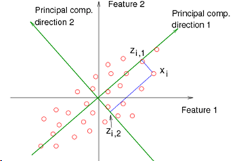
The goal of PCA is to find a direction (line, plane, n-dimensions) in a lower dimension upon which to project the current data, and to find the direction which causes the projection to be as close as possible to the original. So if we have 2 dimensions, we want to find a single line (a number line of 1 dimension) and tilt it at an angle on the 2D graph, then map the 2D points onto positions along that line. For higher dimensional problems, the idea is the same. 3D data is projected onto a 2D plane oriented within the 3D space.
When projecting the point to the (e.g.) line, the movement is done at right angles to the line, and not vertically along the axis, as would be the case in Linear Regression.
In the diagram shown here, direction 1 is better than direction 2, because the point Xi will be mapped to Zi1, which is a smaller movement than if it were mapped to Zi2.
We must perform mean normalization and may need to scale the range of the different features so that they are similar.
We then compute the covariance matrix which tells us far our dataset is spread out, much like the standard deviation. A covariance matrix is a matrix whose element in the i, j position is the covariance between the i th and j th elements. In our case, this is: sumi=1n(X(i) X(i)T)/m or sigma = (X'*X)./m in Octave where X is the data matrix of n dimensions by m samples. A covariance matrix is always symmetric ( A =A' ).
We can use either eig(sigma) or [U,S,V] = svd(sigma) in Octave. U is our covariance matrix. S is a diagonal matrix of singular values which we can use later to compute the compression error.
If k is the number of dimensions we want, (k < n), then take the first k columns of the U matrix and multiply that times the X data matrix. Do not include X0 = 1 offset parameters. So
Ur = U(:,1:k); %reduced subset of U taking first k columns
Z = X * Ur; %new k dimensional data based on original data.
 Expansion
and Error
Expansion
and Error
After finding Ur and Z, we may wish to reproduce a new approximate X, Xa, from those values, which has the original number of dimensions.
Xa = Z * Ur'; %note Ur is transposed
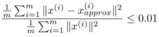
If our dimensional reduction was effective, Xa and X will be close. k should generally be chosen so that the average squared projection error divided by total variation is less than 0.01 as shown by the figure to the right. This error can be calculated for any value of k by summing the S matrix returned by the svd function along the diagonal for k elements, then dividing that by the total diagonal sum of S and subtracting the result from 1. e.g.
1 - ( sum(S(1:k,1:k)(:) / sum(S(:)) )
This allows us to quickly find the value of k which produces the desired total variation. Pro tip, instead of subtracting from 1, just look for the divisor that gives > 0.99.
See also:
Excellent and simple video that explains it in small steps:
| file: /Techref/method/ai/PrincipalComponentAnalysis.htm, 6KB, , updated: 2020/4/3 20:25, local time: 2025/6/2 23:34,
216.73.216.91,10-3-106-20:LOG IN
|
| ©2025 These pages are served without commercial sponsorship. (No popup ads, etc...).Bandwidth abuse increases hosting cost forcing sponsorship or shutdown. This server aggressively defends against automated copying for any reason including offline viewing, duplication, etc... Please respect this requirement and DO NOT RIP THIS SITE. Questions? <A HREF="http://www.sxlist.com/techref/method/ai/PrincipalComponentAnalysis.htm"> Machine Learning Method: Principal Component Analysis</A> |
| Did you find what you needed? |
Welcome to sxlist.com!sales, advertizing, & kind contributors just like you! Please don't rip/copy (here's why Copies of the site on CD are available at minimal cost. |
|
Ashley Roll has put together a really nice little unit here. Leave off the MAX232 and keep these handy for the few times you need true RS232! |
.