Unlike Linear Regression or Logistic Regression, Neural Networks can be applied to Non-linear data or data which would otherwise require to many quadratic features to classify. When there are many features, such as in machine vision problems and especially with Convolution, their combinations can quickly get out of control. NNs have been around since the '50's when they were developed as a way to mimic the operation of the brain. At that time, they were too computationally expensive, but they are making a resurgence given todays computing power.
NN simulate real "neurons" by sending messages to each other. The connections,
xn, are weighted by parameters On,
and the weights are tuned based on experience. There is also an input that
is not from other neurons, x0, called the "bias unit" which is
always set to 1. The weight on the bias unit changes the likelihood that
the neuron will fire irrespective of other inputs. Note: This is still just
y = mX+b. The bias unit is b, (actually
x0 always set to 1, then times O0
so that matrix math is easily applied).
The inputs are X (vector) and the m are the weights
On.
The internal function of a single neuron in the network can be modeled by a simple Logistic unit using an "activation" or "cost" function such as the sigmoid function^ Hyperbolic Tangent^, Rectifier e.g. ReLU (Rectified Linear Unit)^, e.g. max(0,x)^ or SIREN^. In Octave:
g = 1 ./ ( 1 .+ exp(-X*theta) ) ;
Multiple Layers:
![]() NNs can
have multiple layers where the top layer, directly connected to the external
data inputs, is connected through to another layer, which may be connected
to another, and so on before connecting to the final, output, layer. The
inner layers are called hidden layers. Each neuron in a layer is normally
connected to ALL the neurons in the next layer, or to one of a few neurons
or even a single neuron, in the case where the next layers has fewer neurons.
For a multi-class classification NN, with K classes, there would be K output
units and only one would come on at a time. It is common to have a single
neuron on the last, or output, layer. In that case, the computation from
the last layer looks a lot like Logistic Regression. In fact, each layer
is it's own set of mapping input to recognized features.
NNs can
have multiple layers where the top layer, directly connected to the external
data inputs, is connected through to another layer, which may be connected
to another, and so on before connecting to the final, output, layer. The
inner layers are called hidden layers. Each neuron in a layer is normally
connected to ALL the neurons in the next layer, or to one of a few neurons
or even a single neuron, in the case where the next layers has fewer neurons.
For a multi-class classification NN, with K classes, there would be K output
units and only one would come on at a time. It is common to have a single
neuron on the last, or output, layer. In that case, the computation from
the last layer looks a lot like Logistic Regression. In fact, each layer
is it's own set of mapping input to recognized features.
Multiple Parameter Vectors: Because there may be multiple layers,
we must add a new dimension to our vector of parameters
O. The weights on a specific layer (j) may be represented
by O(j) and a specific weight between node (i)
of the prior layer and (i') of the next layer as
Oi'i(j). The activation, or value
computed for output, of a specific neuron (i) in a specific layer (j) can
be represented by ai(j).
ai(j) = "activation" of unit i in layer j. If
a NN has sj units in layer j (not counting any bias units) and
s(j+1) units in layer j+1, and each neuron is connected to every
neuron in the next layer, then O(j) will be
a matrix of s(j+1) by sj + 1. That last "+1" is
because of the bias unit. sj is the number of units not counting
the bias unit.
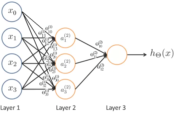 Example
A Neural Net with 3 inputs, x1-x3, a bias unit, x0, a hidden layer with 3 nodes, and a single output, would require the following computations:
a1(2)=g(O10(1)x0
+O11(1)x1
+O12(1)x2
+O13(1)x3)
a2(2)=g(O20(1)x0
+O21(1)x1
+O22(1)x2
+O23(1)x3)
a3(2)=g(O30(1)x0
+O31(1)x1
+O32(1)x2
+O33(1)x3)
h0(x)= a1(3)=
g(O10(2)a0(2)
+O11(2)a1(2)
+O12(2)a2(2)
+O13(2)a3(2))
Notice that the (j) superscript denotes the layer, the subscript
denote the node i within that layer, and in the case of the weights,
O, the first subscript is the node in the higher layer,
and the second is the node in the lower layer. E.g.
O10 is the weight, on a1, of
x0 from the prior layer.
Using Matrix math, the computations that must take place are:
Another way of saying the same thing is:
Note: this example did not include bias units in the hidden layer.
A very simple NN can be made with a single layer consisting of a single neuron
with 2 binary inputs, 1 output, and manually assigned weights to compute
the AND function. The hypothesis function might be:
hO(X) = g( -15x0 + 10x1
+ 10x2 ). Keeping in mind that x0 = 1, and that anything
more than 5 is effectively 1, and less than -5 is 0 from the sigmoid function
g(), we can write the output for all possible input values:
| x1 | x2 | h |
| 0 | 0 | 0 = g(-15) = g(-15·1 + 10·0 + 10·0) |
| 0 | 1 | 0 = g(-5) = g(-15·1 + 10·0 + 10·1) |
| 1 | 0 | 0 = g(-5) = g(-15·1 + 10·1 + 10·0) |
| 1 | 1 | 1 = g(+5) = g(-15·1 + 10·1 + 10·1) |
The binary OR function would be g( -10x0 + 20x1 +
20x2 ). NOT is g( 10 - 20x1 ). Other functions can
be expressed by the same basic formula simply by changing the weights. If
hO(X) = g(
O0x0 +
O1x1 +
02x2 ) Then AND is O
= [-15 10 10] and OR is O = [-10 20 20] and NOT is
O = [10 -20]. NAND is O = [30 -20 -20]
Multiple layers of a NN can be assembled just like multiple gates in a
digital logic circuit. For example,
XOR can be made from 2 layers:
O(1) = [-15 10 10; 10 -20 -20];
O(2) = [-10 20 20]
a1(2) = g( -15x0 + 10x1 +
10x2 ) this is AND
a2(2) = g( 10x0 - 20x1 -
20x2 ) this is NOR (NOT OR)
a1(3) = g( -10a0(2) +
20a1(2) + 20a2(2) ) this is OR
The result is equivalent to XOR = (A AND B) OR NOT(A OR B) where A is x1 and B is x2
Given a two dimensional matrix of weights for a specific layer,
O(l), and the activation of that layer as a vector
a(l), the activation of the next layer, l + 1 is given
by: a(l+1) =
g(O(l)a(l)). Note that for l=1, the
activation is actually the input vector X. However, since bias units don't
get an activation, the size of the l+1 matrix may not match. We can fix this
by breaking the calculation into two steps where we first calculate the
activations for the real nodes in the next layer, and then add a set of bias
units of value 1 to fill out all the nodes for the next cycle:
Note: When propagating from one layer to the next in a NN, it's critical
that the size of the matrix match, including any bias unit columns. For Matrix
multiply or
divide^,
for A*B, the second dimension of A must match the first dimension of B, and
the result will be a matrix which is the first dimension of A by the second
dimension of B.
If A is n x m and B is m x p the result AB
will be n x p. [n x
m]*[m x
p] = [n x
p]
For a 2 layer NN with weights Theta1 and Theta2 for the layers, prediction can be made in Octave:
m = size(X, 1);
a1 = [ones(m, 1) X]; %add a column for bias units
z2 = sigmoid(a1 * Theta1'); %propagate to the inner layer
a2 = [ones(m, 1) z2]; %add a column for bias units
a3 = sigmoid(a2 * Theta2'); %propagate the output layer
[val, p] = max(a3, [], 2); %find the node with the highest output
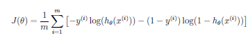
A cost function for a NN can be similar to that for
Logistic Regression:

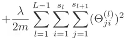
except that there is an additional dimension for the extra units (k). Also, because there are parameters (weights) between each node of the prior layer for each node of the next layer, there are two additional dimensions for the regularization (j,i,l) Note that we still do not include the 0th elements (the bias units) so the indexes start with 1 not 0. Don't confuse that with Octave which starts indexing from 1. In Octave, start the regularization from 2, or zero out index 1 after computing the cost before regularization.
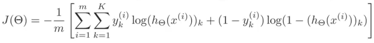
Note this cost function is not convex and can, but rairly does, get stuck at a local minima.
To calculate this cost function, the standard code can be used, but for a classifier NN, we must convert y from individual values, into a set of sets of vectors of zeros and ones where the value is represented by a 1 in the corrisponding location. e.g. if K = 3 and y(m)=2 then class_y(m) = [0; 1; 0]. If y(m) was 1, it would be [1; 0; 0]. To do this (at least for numerical values) we use an identity matrix. In Octave, eye returns an identity matrix. E.g. eye(3) returns [1 0 0; 0 1 0; 0 0 1]. We can index that matrix on both dimensions, returning the y'th row, and all the columns in that row. e.g. eye(3)([2 3 1],:) returns [0 1 0; 0 0 1; 1 0 0] (1 in the 2nd column, 1 in the 3rd column, 1 in the 1st column).
class_y = eye(K)(y,:); %how tricky is that?
costs = -class_y .* log(a3) - (1-class_y) .* log(1-a3);
J = sum(costs(:))/m; %costs is a matrix now. (:) makes a vector.
To calculate the regularization, we must compensate for there being multiple
thetas, and that they are matrixs instead of vectors... and we still need
to cut out the O0 elements (now called bias units).
Theta1(:,2:end) gives us all the rows of Theta1, but leaves out
the first column. (:) turns the resulting matrix into a vector
containing all those elements. This is so the sum doesn't miss the columns
and the element-wise power doesn't care. e.g. for a system with 2 layers:
reg1 = sum(Theta1(:,2:end)(:).^2);
reg2 = sum(Theta2(:,2:end)(:).^2);
J = J + (lambda/(2*m)) * (reg1+reg2);
Note that we sum all the values before multiplying by lambda and dividing by 2m.
TODO: Write a version of this that works for L layers.
Computing the slope of the error for multiple layers is complicated by the
fact that there are many parameters.
Oij(l) vs simply
Oj. We can think about the error of a specific
node j in a specific layer l as
dj(l). For the output
layer L,
dj(L) =
aj(L) - yj or
as a vector of j nodes, d(L) =
a(L) - y Because we are talking about the output layer,
j must be K; the number of outputs. For the earlier layers, again, as a
vector/maxtix (not showing the ij node indexes) we have
d(l) =
(O(l))Td(l+1)
.* g'(z(l)). Note the .* or element wise multiplication.
g'(z(l)) is the derivative (note the ' or "prime" which
means derivative) of the activation function g evaluated at the input functions
given by z(l). Although the math to prove it is very complex, it is know
that g'(z(l)) = a(l) .* (1-a(l)).
There is no
dj(l) for the first
layer. Note that we only have the values needed to calculate the prior layers
after we calculate the later layers, hence the name back propagation. Note
this doesn't include regularization.
Here is the overall method for calculating the gradients in a non-matrix format; there is a loop for each training example, and the vectors inside the loop consider that example only.
Dij(l) = 0 for all l,
i, j. %accumulator
for m = 1:sizeof(y) %for each training
example.
a(1) = x(m) %load
that examples input
for l = 2:L %forward through layers to
output
z(l) = g(
O(l-1)a(l-1) )
%forward_propagate
a(l) = [1's z(l)]
%add bias units
d(L) =
a(L) - y(m) %error for this
examples output
for l = L-1:2 %backward through hidden
layers
d(l) =
O(l)Td(l+1)
.* (
a(l).*(1-a(l)) )
%? calculate partial derivative for all i,
j.
Dij(l) :=
Dij(l) +
aj(l)Tdi(l+1)
%accumulate partial derivatives
% in vector form
D(l) :=
D(l) +
d(l+1)
a(l)T
Dij(l) := 1/m
(
Dij(l) + lambda
Oij(l) ) if j is not 0
Dij(l) := 1/m
Dij(l) if j is 0
%don't regularize bias term.
Note that the delta values for the backwards propagation can be calculated
to simplify the matrix math, but they will be disgarded duing forward
propagation. The matrix multiplication
d(l+1)
O(l) is summing, for
example, d1(l+1)
O12(l) +
d2(l+1)
O22(l) so again,
? we must transpose
O(l) to make the matrix line up. Also, for
di(l+1)aj(l)
in matrix form
d(l+1)a(l) we must transpose
a(l)
Here is an Octave matrix implementation for a NN with 3 layers:
d3 = a3 - class_y;
d2 = d3 * Theta2(:,2:end); %dont include bias units column
d2 = d2 .* (z2 .* (1-z2)); %partial derivative
% z2 excludes bias column. Could use a2 and all Theta2 & remove first column
grad1 = (d2' * a1) ./ m;
grad2 = (d3' * a2) ./ m;
To regularize the gradients, simply scale O by lambda /
m while avoiding the bias units. e.g.
Theta1(:,1) = 0; %remove bias units.
grad1 = grad1 + (Theta1 .* (lambda/m));
The theta and gradient values are no longer vectors, but are now matrixes. The D or delta's also matrix. To use standard regression algorithems like fminunc etc... we must "unroll" them into vectors. For example, in a 3 layer vector, if there are 10 units in the first two layers and 1 in the last.
thetaVec = [ Theta1(:); Theta2(:); ... ]
gradVec = [ grad1(:); grad2(:); ... ]

Theta1 = reshape(thetaVec(1:110), 10, 11]
Theta2 = reshape(thetaVec(111:220), 10, 11]
Theta3 = reshape(thetaVec(221:231), 1, 11]
This is a diagnostic technique to make sure that your implementation of the gradient part of the cost function is valid. To validate Dij(l), we can take the value of the cost curve at a point just past and just before the point and one value should be more, while the other value should be less. This should be familiar as part of the definition of how derivatives are calculated. In Octave:
s_guess = (cost(theta + e) - cost(theta - e)) / (2*e); %approximate derivative of J(theta)
We can make such an estimate for each element of a vector theta, by computing the estimate for the cost function once per element, but with only that one element being "tweaked" by e.
for i = 1:num_parms
  theta_up = theta; theta_up(i) = theta_up(i)+e;
  theta_dn = theta; theta_dn(i) = theta_dn(i)-e;
  s_guess(i) = (cost(theta_up) - cost(theta_dn)) / (2*e);
If all the theta weights are set to the same value, then all the errors will be the same, and all the back propagation corrections will be the same, and so on. It is critically important that the initial values are different so they can further differentiate in the correct directions. Random values work well. The range should be some small value distributed around zero. The range can be based on the number of units in the network. e.g. sqrt(6)/sqrt(sum(s())). In Octave:
ThetaJ = rand(s(j),s(j)+1) * (2*init_e) - init_e;
Inputs: Number of features
Outputs: Number of classifications
Hidden layers: Start with one. Make each hidden layer the same size; same number of units. More units is better, but expensive. More units in the hidden layers than input.
The Gaussian Kernel SVM may be better for small feature sets ( n < 1000 ) and reasonable sample sets ( 10 < m < 10,000 ). Logistic or Linear Regression may be better for simpler problems with very large training sets or features.
Also:
Fuzzy Logic and neural networks are two design methods that are coming into favor in embedded systems. The two methods are very different from each other, from conception to implementation. However, the advantages and disadvantages of the two can complement each other.The advantage of neural networks is that it is possible to design them without completely understanding the underlying logical rules by which they operate. The neural network designer applies a set of inputs to the network and "trains" it to produce the required output. The inputs must represent the behavior of the system that is being programmed, and the outputs should match the desired result within some margin of error. If the network's output does not agree with the desired result, the structure of the neural network is altered until it does. After training it is assumed that the network will also produce the desired output, or something close to it, when it is presented with new and unknown data.
In contrast, a fuzzy-logic system can be precisely described. Before a fuzzy control system is designed, its desired logical operation must be analyzed and translated into fuzzy-logic rules. This is the step where neural networks technology can be helpful to the fuzzy-logic designer. The designer can first train a software neural network to produce the desired output from a given set of inputs and outputs and then use a software tool to extract the underlying rules from the neural network. The extracted rules are translated into fuzzy-logic rules.
Fuzzy logic is not a complete design solution. It supplements rather than replaces traditional event control and PID (proportional, integral, and derivative) control techniques. Fuzzy logic relies on grade of membership and artificial intelligence techniques. It works best when it is applied to non-linear systems with many inputs that cannot be easily expressed in either mathematical equations used for PID control or IF-THEN statements used for event control.
In an effort to change fuzzy logic from a "buzzword" (as it is in most parts of the world) to a well established design method (as it is in Japan), most manufacturers of microcontrollers have introduced fuzzy logic software. Most software generates code for specific microcontrollers, while other generates C code which can be compiled for any microcontroller.
See also:
| file: /Techref/method/ai/NeuralNets.htm, 32KB, , updated: 2023/8/20 10:48, local time: 2025/7/1 04:04,
216.73.216.243,10-1-246-116:LOG IN
|
| ©2025 These pages are served without commercial sponsorship. (No popup ads, etc...).Bandwidth abuse increases hosting cost forcing sponsorship or shutdown. This server aggressively defends against automated copying for any reason including offline viewing, duplication, etc... Please respect this requirement and DO NOT RIP THIS SITE. Questions? <A HREF="http://www.sxlist.com/techref/method/ai/NeuralNets.htm"> Machine Learning, Neural Networks Method</A> |
| Did you find what you needed? |
Welcome to sxlist.com!sales, advertizing, & kind contributors just like you! Please don't rip/copy (here's why Copies of the site on CD are available at minimal cost. |
|
The Backwoods Guide to Computer Lingo |
.