Anomaly Detection answers questions of the type: Is a data point like the other data points in the set, or is it far enough out of the others to raise concern? It is used to reject products that are likely to fail, to look for outliers, to identify subjects that are behaving strangely, devices about to fail, etc... We could use a learning system like a Logistic Classifier, but because, by definition, there are few anomalous data points, checking against the Normal Distribution can avoid accuracy vs precision/recall issues and still detect previously unseen anomalies of many different types.
 Gaussian (Normal) Distribution
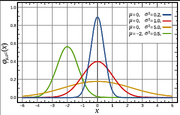
If the probability distribution of X is Gaussian^ (aka Normal) with mean (µ or mu) and variance sigma squared (ó2 or sigma2) we write X ~ N(µ, ó2). {ed, using ó as the greek letter sigma}. µ gives us the center of the normal bell curve, ó is the standard deviation^ or width from the center of the curve to the inflection point^ where the slope of the curve changes from concave to convex. ó2 is the variance.
In the figure here, the red line is the Normal distribution.
Estimating: µ can be estimated as the average value of X. ó2 is the average of X .- µ
We can do this for each individual feature of a dataset as follows:
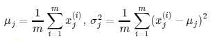
We do this for all features. If there are n features, j = 1:n. As a vector,
µ = mean(X(i)); ó2 =
mean(X(i) - µ); As a matrix
of many features, in Octave:
mu = mean(X,1); %operate only along the first dimension
sigma2 = var(X,1,1); %var is close enough
%Note: the first 1 is OPT (option), which selects 1/m instead of 1/(m-1)
Given a new data point, we can compare it's features to the µ and
ó2 of the other features
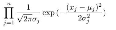
if this value (called the Probability Density, p) is greater than
some threshold, e or epsilon, the data point is anomalous. e.g. y=1.
Below the threshold, it is not, e.g. y=0.
One problem with the Normal system used above is that when the axis are somewhat related, e.g. power use and temperature (a device under load often consumes more power and runs a little hot), a datapoint can fall at the low end of one axis and at the high end of another... when plotted on the separate axis, it might not be outside of the acceptable range for either axis, e.g. devices sometimes consume little power, and sometimes get hot... but the combination places it well outside the grouping of data we have seen before. e.g. a unit running hot while at the same time consuming little power is abnormal. We can compinsate for this in the standard model by manually creating a new feature such as X3 = X1/X2 where X1 might be power use, and X2 might be heat. Multivariate Gaussian Distribution can look for the combination of factors which are unusual together.
Instead of modeling each feature separately, we will model them all together by making sigma a matrix. By changing the values in this nxn version of sigma, we can control the distribution for different axis individually. For example if sigma = [1 0; 0 0.6] then X1 has a Normal distribution of 1, and X2 of 0.6 meaning that X2 is expected to take on a more narrow range of values. If sigma = [1 0.5; 0.5 1] then X1 and X2 cover the same range, but now we are modeling correlations between the axis; we are saying that when X1 is large, we expect X2 to be large as well. The correlation is controlled by the size of the value; if sigma = [1 0.8; 0.8 1] then we are saying that X1 and X2 are strongly correlated and if X1 is large and X2 is small, that should fall outside our limit and trigger an alarm. Negative values indicate an inverse correlation; we expect X1 to be large when X2 is small.
Our new probablity density function is actually very close to the old one:
(in fact, it's the same, if you constrain it such that the axies are aligned
i.e. where sigma is a diagonal matrix.)
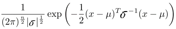
but we have rearranged terms to make it easier to compute as a matrix.
ó -1is the same as 1/ó. In matrix
form, the |ó| can be calculated in
Octave as det(sigma) where
sigma is an nxn matrix. µ is an n dimensional vector.
As before, we are training µ = mean(X(i)) but now ó2 = mean( (X(i) - µ)(X(i) - µ)T );
So the advantage here is that it will automatically find correlations between features. It is, however, more computationally expensive, and does not scale as well as the standard Normal model. It also doesn't work as well unless m > n (because ó will be non-invertable) and perhaps m should be 10 or more times n in practice. ó can also be non-invertable if you have redundant features, so carefully selecting features is important.
In Octave:
k = length(mu);

if (size(Sigma, 2) == 1) || (size(Sigma, 1) == 1)
    Sigma = diag(Sigma);
    end

X = bsxfun(@minus, X, mu(:)');
p = (2 * pi) ^ (- k / 2) * det(Sigma) ^ (-0.5) * ...
    exp(-0.5 * sum(bsxfun(@times, X * pinv(Sigma), X), 2));
Select features which appear to fit the Normal distribution. The histogram plot (in Octave, use the hist command) can be helpful to visualize each features data. For important features, we might be able to "correct" the distribution by applying some sort of transform. E.g. if the histogram shows data skewed to the lower end of the scale, try using log(Xj) or take the square root (or some other power) to make a training feature which is more gaussian in shape.
We can also do error analysis on each feature to see which are more or less correlated with anomalies.
In most cases, by definition, training data will have many examples which are not-anomalous (y=0) and only a few which are (y=1). We can train the µ and ó2 data from a sub set of the non-anomalous data then build a cross validation and test sets which split the anomalous examples and have the standard fractions of non-anomalous examples. Train on the training data (with no anomalous examples) then test against the CV and test sets.
Be sure to check false positives and negatives as well as true positives and negatives because the data is typically skewed. A machine that always predicts y=0 would have high accuracy.
Use the cross validation set to choose the parameter for e, the threshold by calculating the F1 score for many values of e between the minimum and maximum values of the data.
stepsize = (max(p) - min(p)) / 1000;
for epsilon = min(p):stepsize:max(p)
  predictions = (p < epsilon);
  F1 = findF1(predictions, epsilon); % see Skewed Classes
  if F1 > bestF1
    bestF1 = F1;
    bestEpsilon = epsilon;
    end
  end
Given the probability density (p) and a good value for our cut off point (epsilon) we can now easily find our outliers:
outliers = find(p < epsilon);
| file: /Techref/method/ai/AnomalyDetection.htm, 8KB, , updated: 2019/1/29 23:17, local time: 2025/6/7 17:26,
216.73.216.34,10-3-44-153:LOG IN
|
| ©2025 These pages are served without commercial sponsorship. (No popup ads, etc...).Bandwidth abuse increases hosting cost forcing sponsorship or shutdown. This server aggressively defends against automated copying for any reason including offline viewing, duplication, etc... Please respect this requirement and DO NOT RIP THIS SITE. Questions? <A HREF="http://www.sxlist.com/techref/method/ai/AnomalyDetection.htm"> Machine Learning, Anomaly Detection Method</A> |
| Did you find what you needed? |
Welcome to sxlist.com!sales, advertizing, & kind contributors just like you! Please don't rip/copy (here's why Copies of the site on CD are available at minimal cost. |
Welcome to www.sxlist.com! |
.